Area Under Receiver Operating Characteristic curve (AUROC)

What is it?

AUROC (or implicitly shorten by AUC) is a metric to evaluate and compare the classification performance of machine learning models.

Why not just use accuracy? Let review some basic definitions

Accuracy is commonly used, but somtimes it is not enough to reflect the efficiency of the models. Let review some basic definitions of binary-class prediction:

• True Positive (TP): when you predict a Positive sample as Positive. (Correct)
• False Negative (FN): when you predict a Positive sample as Negative. (Incorrect)
• False Positive (FP): when you predict a Negative sample as Positive. (Incorrect)
• True Negative (TN): when you predict a Negative sample as Negative. (Correct)

In short, TP, FN, FP, TN is defined by [Correct (True)/Incorrect (False) ][Prediction Label].

• Accuracy (Acc):

\[Acc = \frac{\text{Number of Correct Prediction}}{\text{Number of total samples}} = \frac{TP + TN}{TP+TN +FP +FN}\]

• True Positive Rate ( or Sensitivity)(TPR) :

\[TPR = \frac{\text{Number of Correct Predicted Positive}}{\text{Number of total Positive samples}} = \frac{TP}{TP+ FN}\]

• False Positive Rate ( or Fall-out)(FPR) :

\[FPR = \frac{\text{Number of Incorrect Predicted Positive}}{\text{Number of total Negative samples}} = \frac{FP}{TN+ FP}\]

Usually, the predictor, e.g. linear regression, outputs the probability of a sample belong to the Postive class, e.g. \(P(x \in \text{Positive}) = p\). And we predict a sample as Positive if \(p \geq T\), else Negative. Hence, by varying the threshold \(T\), we affect the TFR,TPR and Acc:

• Specifically, increasing \(T\) makes predictor more concervative, hence FPR reduces (which is good), but TPR also reduces (which is bad).
• In contrast, reducing \(T\) makes predictor more agressive, hence FPR increases (which is bad), but TPR also increases (which is good).
• Changing of \(Acc\) is not monotonic as TFR and TPR when changing the threshold (this is not good).
• When choosing the threshold, we compromise between Sensitivity and Fall-Out.

How is it defined? What are the advantages?

So, if for each threshold value \(T\), we plot a point (TFR on x-axis, TPR on y-axis), we get the Receiver Operating Characteristic (ROC) curve. Hence, by computing the Area Under this Curve (AUC), we can merge the two metrics TFR and TPR into one metric AUROC, that is independent to the threshold, as illustrated in the Fig. 1.

• The higher AUROC, the better predictor is. The perfect predictor has \(AUROC =1.0\).
• The center line is at the chance level.
• ROC Curves can be used to evaluate the tradeoff between true- and false-positive rates of classification algorithms.
• ROC Curves are insensitive to class distribution. If the proportion of positive to negative instances changes, the ROC Curve will not change.
• If you have \(C\) classes, use One-vs-All to convert the problem to \(C\) binary classes.

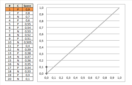
Figure 1. Example of AUROC ([1])

How to compute it?

Let say you apply the prediction to all test samples, here are the steps:

1. Rank the samples by their score \(p\) from highest to lowest. The middle column \(C\) contains the true label of the sample.
2. Moving from top to the bottom of the table, and from (0,0) of the plot. At each sample, choose a threshold equal to its score \(p\)
   • If \(x\) is Postive, we add 1 more Possive sample. That means, the TPR increases by \(\delta y= \frac{1}{\text{Number of Positive samples}}\). On the plot, move up by \(\delta y\)
   • If \(x\) is Negative, we add 1 more Negative sample. That means, the FPR increases by \(\delta x= \frac{1}{\text{Number of Negative samples}}\). On the plot, move right by \(\delta x\)

And then we compute the Area Under this curve.

In python, this is much easier:

  from sklearn.metrics import roc_auc_score

  # y_true is a True label of the sample (Binary class)
  y_predict = Predict_funct(x) # y_predict is the probability (score) predicted
  auroc = roc_auc_score(y_true, y_predict)

How to select the best threshold to yield highest accuracy?

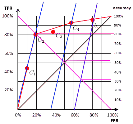
Let \(N\) be the total number of samples, \(POS\) and \(NEG\) be the number of postive and negative sample, respectively. Define \(pos= POS/N\) and $$neg = NEG/N$, the acuracy can be rewritten as:

\[Acc = \frac{TP+TN}{N}= \frac{TP}{POS}\frac{POS}{N} + \frac{TN+FP-FP}{NEG}\frac{NEG}{N} = TPR.pos + (1-FPR).neg\]

Hence

\[TPR = \frac{neg}{pos} FPR + \frac{Acc - neg}{pos}\]

Thus, a line with the slope \(a= \frac{neg}{pos}\) and goes through the point (TFR, TPR) of the ROC curve. The intersection with the ISO line shows the accuracy, as illustrated as:

<<<<<<< HEAD

Figure 2. Select best accuracy for a=4 ([1])

=======

</h4> Figure 2. Select best accuracy for a=4 ([1]) </h4>

>>>>>>> master

Reference

[1] http://mlwiki.org/index.php/ROC_Analysis