t-SNE: STOCHASTIC NEIGHBOR EMBEDDING A Visualization tool for high dimension data

What is this?

t-SNE is a method to display data from high dimensional space into 2D or 3D space, so that we can have a sense of how the data is distributed, e.g, how data from different class are separated.

Why not just use PCA? Let review some basic definitions

The process of mapping data from high dimensional space $X \in \Re^{n}$ to the lower one $Y \in \Re^{m}, m<n $ is called Embedded Mapping. This process is often used when we want to extract most useful features from the data, and remove trivial (or noise) features.

PCA is an most popular unsupervised method that aims to find a linear map $W$: $y=W x$ so that the projected data are most separated in the new Embedded space $Y$. That means the variance of the data after mapping are maximized. Mathematically,this is obtained by

\[W= {\rm argmax~} C(W), \hspace{0.1in} C(W)=\frac{y^Ty}{\|W\|^2} = \frac{W^T X^T X W}{W^T W}\]

For feature dimension reduction, we can pickup the first $m$ features, since they have higher variance than the later one. And this is GOOD.

For visualization, however, we can only pickup maximum the first 3 components for XYZ display. Doing so, we accept to lose many information, and this is INSUFFICIENT.

In short, PCA only cares about the distance between the points, and try to maximize the variance of data.

STOCHASTIC NEIGHBOR EMBEDDING (SNE)

For display data, we care more about the local structure of data, rather than the distance between them.

We want to find a map such that if the points are close (or far away) in the original data, they should be close (or far away) in the embedded data. Thus, SNE proposes a method where the bridge between the two spaces is the probability that we can find the neighbor points of a given point data.

Mathematically, if $p_{j|i}$ is the probability that we can find a neighbor point $x_j$ of a point $x_i$ in the original space, and $q_{j|i}$ is the probability that we can find neighbor $y_j$ of a point $y_i$, we want $p_{j|i} \approx q_{j|i}$. Since $p_{j|i}$ and $q_{j|i}$ are the probability, Kullback Leiber distance is more suitable to measure their difference, and the cost function can be constructed as:

\[C=\sum_i KL(P_i\|Q_i) =\sum_i \sum_j p_{j|i} \log \frac{p_{j|i}}{q_{j|i}}\]

If it is perfect match, e.g. $p_{j|i} = q_{j|i}$, then $C=0$.

Now, the next question is how to build $p_{j|i}$ and $p_{j|i}$? For nearby data, e.g. if $p_j$ is inside a sphere centered at $p_i$ with radius $\sigma_i$, $p_{j|i}$ should be high. If it is far from the center, its probability should be low. Thus, a bell-shape distribution , particularly Gaussian, should be used:

\[p_{j|i}= \frac{\exp(-\|x_i -x_j \|^2/2\sigma_i^2)}{\sum_{k} \exp(-\|x_i -x_k \|^2/2\sigma_i^2)}\]

Similarly, we do construct $p_{j|i}$ in the same way, except that we can further simplify the formula by re-scaling $\sigma_i$ to $1/\sqrt{2}$, thus

\[q_{j|i}= \frac{\exp(-\|y_i -y_j \|^2)}{\sum_{k} \exp(-\|y_i -y_k \|^2)}\]

The last thing to complete the formulation is find $\sigma_i$ for each datapoint $x_i$ in the original dimension, but let skip it for now.

Finally, the point $y_i$ can be find by Gradient descent method with momentum term, such that: $Y^{(t)} = Y^{(t)} + \eta \frac{\delta C}{\delta Y} + \alpha(t)(Y^{(t-1)} - Y^{(t-2)})$ where $\eta$ is the learning rate, $\alpha$ is the momentum coefficient, and the cost function gradient:

\[\frac{\delta C}{\delta y_i} = 2\sum_j (p_{j|i} - q_{j|i} + p_{i|j} -q_{i|j})(y_i-y_j)\]

Each component of the gradient $\frac{\delta C}{\delta Y}$ can be physically explained as the force of spring, where the length is $(y_i-y_j)$, and the stiffness is $(p_{j|i} - q_{j|i} + p_{i|j} -q_{i|j})$. If $p_{j|i}+p_{i|j}>q_{j|i}+q_{i|j}$, then $y_i$ and $y_j$ is pushed farther, and vice versa, until the stiffness is 0.

Student Distribution STOCHASTIC NEIGHBOR EMBEDDING (t-SNE)

SNE Symmetric: Replacing conditional distribution $p_{i|j} + p_{j|i}$ by symmetric join distribution $p_{ij}$

The author proposed a slight modification of the probability :

\[q_{ji}= \frac{\exp(-\|y_i -y_j \|^2)}{\sum_{k \neq l} \exp(-\|x_k -x_l \|^2)}, \hspace{0.5in} p_{ij} = \frac{p_{j|i} + p_{i|j}}{2n}\]

to simplify the gradient form to :

\[\frac{\delta C}{\delta y_i} = 4\sum_j (p_{ij} - q_{ji})(y_i-y_j)\]

Student t-SNE: Replacing Gaussian distribution in Output Space by t-distribution

The output distribution is replaced by t-distribution:

\[q_{ij} = \frac{(1 + \|y_i -y_j \|^2)^{-1}}{\sum_{k \neq l} (1 + \|y_k -y_l \|^2)^{-1}},\]

Hence, the gradient becomes

\[\frac{\delta C}{\delta y_i} = 4\sum_j (p_{ij} - q_{ji})(y_i-y_j)(1 + \|y_i -y_j \|^2)^{-1}\]

t-SNE algorithm

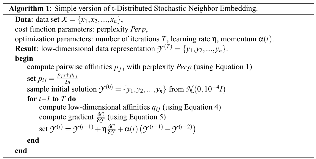
How to Use t-SNE Effectively

To decide the Gaussian window $\sigma_i$, there is a tuneable parameters, named perplexity, which loosely, a guess about the number of close neighbors each point has. Keep in mind the following things when using t-SNE:

1. Perplexity is important, eventhough the author suggests the safe range is [5-50].
2. Multiple runs give the same global shape
3. Cluster sizes in a t-SNE plot mean nothing
4. Distances between clusters might not mean anything
5. Random noise doesn’t always look random.
6. You can see some shapes, sometimes
7. For topology, you may need more than one plot

Reference:

[1] Van Der Maaten, L. J. P., & Hinton, G. E. (2008). Visualizing high-dimensional data using t-sne. Journal of Machine Learning Research, 9, 2579–2605. https://doi.org/10.1007/s10479-011-0841-3

[2] Maaten, L. Van Der. (2009). Learning a Parametric Embedding by Preserving Local Structure. JMLR Proceedings Vol. 5 (AISTATS), 384–391.

[3] Van Der Maaten, L., & Hinton, G. (2012). Visualizing non-metric similarities in multiple maps. Machine Learning, 87(1), 33–55. https://doi.org/10.1007/s10994-011-5273-4